Fast-track course on linear algebra for scientists and engineers.
Linear Equations
Many science and engineering relationships can be modeled as linear systems such as circuit analysis, structural analysis, and analytical chemistry (articles and projects for each of these subjects will be released soon, so stay tuned!). It is therefore very important to build a strong foundation in linear systems. A linear equation is an equation which takes an input and the output follows a linear trajectory. Suppose a linear function with input x and output y , then this can be expressed using the following forms:
Standard Form
Ax+By+C=0
Where A, B, and C are constants. This is the general equation because it is similar to the standard form of a conic equation, which is used for more interesting functions such as parabolas (also referred to as quadratics), hyperbolas, circles, and ellipses. To simplify this equation, we can subtract the constant C from both sides of the equation and so the following is also an equivalent expression of the standard form \to Ax+By=-C. Since C is simply a constant, we can neglect the negative sign, as this can be included within the constant, so the simplified standard form is Ax+By=C.
Slope-Intercept Form
y=mx+b
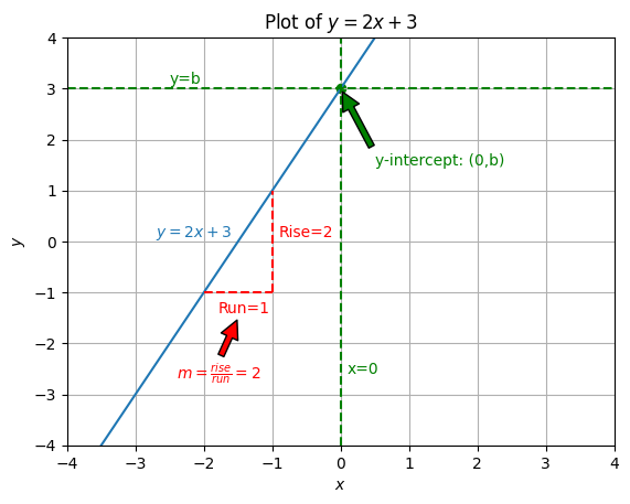
Where m is the slope of the line, and b is the y-intercept. The y-intercept is the value of y at the point where x=0 . To understand this equation intuitively, this graph shows how to obtain the equation of a line:

As you can see in the graph, we obtain the y-intercept by seeing what y-value intersects with the line at x=0 . This y-value is our y-intercept, which is b in the slope form equation. To obtain the slope we find two points on the line and calculate the change in the y and x direction, also referred to as the rise and run respectively. In this graph, for example, I selected the points (x=-2,y=-1) and (x=-1,y=1) , so the change in the x-direction is given as \Delta x = x_2 - x_1 = (-1) - (-2) = 1 and the change in the y-direction is given as \Delta y = y_2 - y_1 = (1) - (-1) . Then, the slope is calculated using by dividing the rise by the run \to \frac{\Delta y}{\Delta x}=2. The slope yields our m value.
Point-Slope Form
y-y_1=m(x-x_1)
Where you are given the point (x_1,y_1) and the slope m . This equation is useful if you are given a point rather than the y-intercept. If you use one of the points (x=-1,y=1) from linear function f(x)=y=2x+3 of the above example, you can see that you can arrive at the slope-intercept form from the point-slope form.
y-1=2(x-(-1))
y-1+1=2(x-(-1))+1\to y = 2(x+1)+1
\boxed{y=2x+3}
Linear Systems
In the above examples, we considered a linear equation with only one variable: x . When you have linear equations with multiple variables, the equation can be written as follows:
a_1x_1+a_2x_2+a_3x_3+\dotsm+a_nx_n = b
Where a_1, a_2, a_3,...,a_n are constant multipliers (referred to as coefficients) for the variables x_1,x_2,x_3,...,x_n and b is a constant, for any amount of variables n . This is only one equation, but multiple variables are included. When you have multiple linear equations, then you have a system of linear equations or simply a linear system. Let’s consider a simple linear system: a system of two equations with two variables x_1, x_2 :
\begin{align*} x_1 + x_2 &= 1\\ 2x_1-x_2&=0 \end{align*}
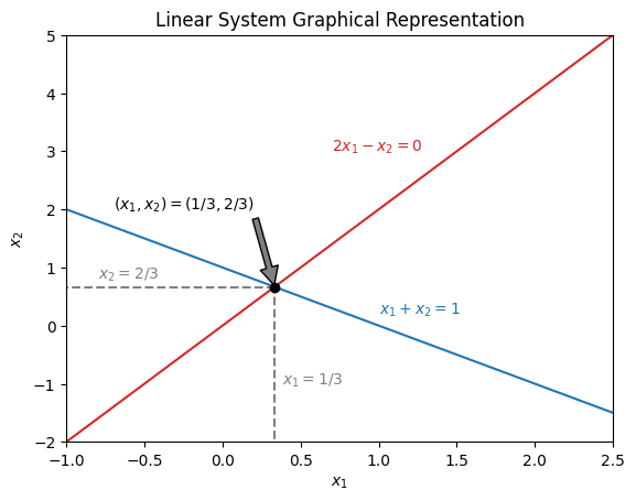
The graphical representation of this system is given below:

The solution of the linear system is the point at which both lines intersect. From the graphical representation, we can see that the solution of the system is at the point (x_1,x_2)=\left(\frac{1}{3},\frac{2}{3}\right) . To arrive at this solution algebraically, one option is to employ Gaussian elimination.
Gaussian Elimination
Gaussian elimination manipulates the system to eliminate one of the variables, allowing us to solve for the remaining variable. The solution can then be substituted back into either of the two initial equations to solve for the eliminated variable. In this example, let’s eliminate x_1 . Recall that any manipulation to the equation, when done to both sides of the equation (left and right of the equal sign), will return an equivalent equation. Therefore, we can multiply both sides of the first equation by 2 and then subtract the second equation:
Elimination
\begin{align*} 2\times(x_1 + x_2) = 2\times(1) \to \cancel{2x_1}+2x_2&=2 \\ -(\cancel{2x_1} - x_2 &=0) \\ \hline 3x_2 &= 2 \end{align*} \\ \boxed{x_2=2/3}
Back Substitution
\begin{align*}x_1+x_2=1\xrightarrow{x_2=2/3} x_1+2/3=1 \\ \hline\\ \end{align*}\\ \boxed{x_1=1/3}
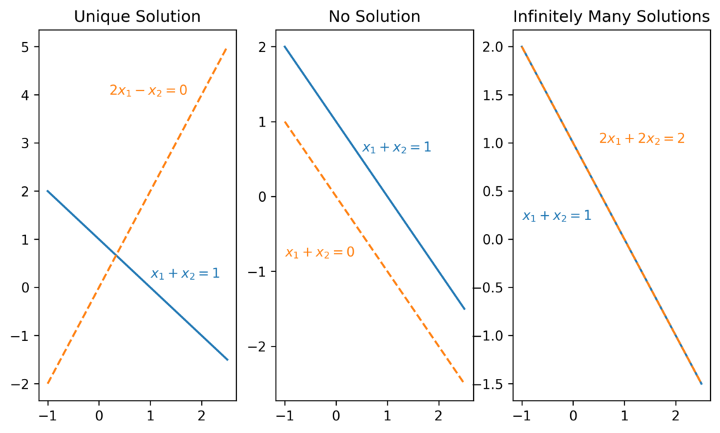
In this case, we arrive at a single unique solution, meaning the lines do not intersect at any point other than (1/3,2/3) . The only other possible cases are linear systems with infinitely many solutions or linear systems with no solution. Example graphical representations for all three possible cases are given below:

While solving linear systems graphically or via Gaussian elimination will yield the correct result, linear systems can become difficult and time-consuming to solve in these ways when you have many variables. Another way to solve linear systems which scales up and makes it easier to solve larger systems involves the use of matrices and vectors. In the following section we will define these mathematical tools and their properties.
Intro to Matrices and Vectors
A matrix (plural is matrices) is a rectangular array of numbers or functions with dimensions of m rows and n columns which is enclosed in brackets and is typically denoted symbolically by bold capitalized variables. Let’s take a look at matrix \mathbf{A}:
\mathbf{A} = \begin{bmatrix} a_{11} & a_{12}\\ a_{21} & a_{22} \end{bmatrix}
Matrix \mathbf{A} has dimensions of 2\times2 so two rows and two columns. In this matrix, we have 4 numbers a_{11},a_{12},a_{21},a_{22} , which have subscripts giving their index. An index tells the exact position of a value inside a matrix. So a_{11} is the value a at the index m=1 and n=1 , which means the value located in the first row and the first column. a_{12} is the value located in the first row and the second column, and so on. The following matrix \mathbf{B} is a 2\times3 matrix:
\mathbf{B} = \begin{bmatrix} b_{11} & b_{12} & b_{13} \\ b_{21} & b_{22} & b_{23} \end{bmatrix}
Some important matrix patterns to learn and are frequently encountered in engineering and science applications are the zero matrix, identity or unity matrix, upper triangular matrix, lower triangular matrix, and scalar matrix.
| Zero Matrix (\mathbf{0}) | Identity Matrix (\mathbf{I}) | Upper Triangular Matrix (\mathbf{U}) |
| \mathbf{0} = \begin{bmatrix} 0 & 0 & \dotsm & 0 \\ 0 & 0 & \dotsm & 0 \\ \vdots & \vdots & \ddots & \vdots \\ 0 & 0 & \dotsm & 0 \end{bmatrix}_{n\times n} | \mathbf{I} = \begin{bmatrix} 1 & 0 & \dotsm & 0 \\ 0 & 1 & \dotsm & 0 \\ \vdots & \vdots & \ddots & \vdots \\ 0 & 0 & \dotsm & 1 \end{bmatrix}_{n\times n} | \mathbf{U} =\begin{bmatrix} a & b & c \\ 0 & d & e \\ 0 & 0 & f\end{bmatrix}_{n\times n} |
| Lower Triangular Matrix (\mathbf{L}) | Scalar Matrix (\mathbf{K}) |
| \mathbf{L} = \begin{bmatrix} a & 0 & 0 \\ b & c & 0 \\ d & e & f\end{bmatrix}_{n\times n} | \mathbf{K} = \begin{bmatrix} k & 0 & \dotsm & 0 \\ 0 & k & \dotsm & 0 \\ \vdots & \vdots & \ddots & \vdots \\ 0 & 0 & \dotsm & k \end{bmatrix}_{n\times n} |
A matrix with dimensions m\times1 or 1\times n is called a column vector or a row vector, respectively. A vector is denoted as a lowercase bold letter, a lowercase letter with an arrow on top, or both:
\text{Column Vector: } \mathbf{x}=\vec{x} = \begin{bmatrix} x_1 \\ x_2 \\ x_3 \\ x_4 \\ \vdots \\ x_m \end{bmatrix}
\text{Row Vector: }\mathbf{x}=\vec{x} = \begin{bmatrix} x_1 & x_2 & x_3 & x_4 & \dotsm & x_n \end{bmatrix}
Alternatively, a vector can be represented as a bracketed list of values. In this case whether the vector is a column or row vector depends on the context in which it is used. In many mathematical and engineering contexts, vectors are typically represented as column vectors, but it’s essential to be aware that different disciplines or applications may follow different conventions. For notational convenience, column vectors are frequently written horizontally in angular brackets.
\text{Alternative Representation of Column Vector: } \mathbf{x}=\vec{x} = \braket{x_1, x_2, x_3, ..., x_i}
We can perform mathematical operations with matrices using the following definitions and rules[1]:
Addition of Matrices
The sum of two matrices \mathbf{A} and \mathbf{B} of the same size is written \mathbf{A} + \mathbf{B} and has the entries obtained by adding each element of \mathbf{A} to the element of the same index \mathbf{B} .
Addition Rules
\begin{align} \mathbf{A}+\mathbf{B}&=\mathbf{B}+\mathbf{A} \\ (\mathbf{A}+\mathbf{B})+\mathbf{C} &= \mathbf{A} + (\mathbf{B}+\mathbf{C}) \\ \mathbf{0} + \mathbf{A} &= \mathbf{A} &\\ \mathbf{A} + (-\mathbf{A}) &= \mathbf{0} \end{align}
Example
\mathbf{A} = \begin{bmatrix} -4 & 6 & 3 \\ 0 & 1 & 2 \end{bmatrix}_{m\times n=2\times3}
\mathbf{B} = \begin{bmatrix} 5 & -1 & 0 \\ 3 & 1 & 0 \end{bmatrix}_{m\times n=2\times3}
\mathbf{A}+\mathbf{B}=\begin{bmatrix} (-4+5) & (6-1) & (3+0) \\ (0+3) & (1+1) & (2+0) \end{bmatrix}=\begin{bmatrix} 1 & 5 & 3 \\ 3 & 2 & 2 \end{bmatrix}
\boxed{ \mathbf{A}+\mathbf{B}=\begin{bmatrix} 1 & 5 & 3 \\ 3 & 2 & 2 \end{bmatrix}}
Scalar Multiplication
The product of any m\times n matrix \mathbf{A} and any scalar (constant multiplier) c is written c\mathbf{A} and is obtained by multiplying each element of \mathbf{A} by c .
Scalar Multiplication Rules
\begin{align} c(\mathbf{A}+\mathbf{B})&=c\mathbf{B}+c\mathbf{A}\\ (c+k)\mathbf{A}&=c\mathbf{A}+k\mathbf{A}\\c(k\mathbf{A}) &= (ck)\mathbf{A} \\ 1\mathbf{A} &= \mathbf{A} \end{align}
Example
\mathbf{A} = \begin{bmatrix} 1 & 4 \\ 5 & 2 \\ 9 & 3 \end{bmatrix}
c=2
c\mathbf{A} = \begin{bmatrix} (1\times2) & (4\times2)\\ (5\times2) & (2\times2) \\ (9\times2) & (3\times2) \end{bmatrix} = \begin{bmatrix} 2 & 8 \\ 10 & 4 \\ 18 & 6 \end{bmatrix}
\boxed{c\mathbf{A} = \begin{bmatrix} 2 & 8 \\ 10 & 4 \\ 18 & 6 \end{bmatrix}}
Matrix Multiplication
The product \mathbf{C}=\mathbf{AB} (in this order) of an m\times n matrix \mathbf{A} times an r\times p matrix \mathbf{B} is defined if and only if r = n. The resulting product is an m\times p matrix \mathbf{C} .
\begin{array}{cccc} \mathbf{A} & \mathbf{B} &= &\mathbf{C}\\ [m\times n]& [r\times p] &=& [m\times p] \end{array}
The entries of the resulting product \mathbf{C} is obtained by multiplying each entry in the j th row of \mathbf{A} by the entry in the k th column of \mathbf{B} and then summing these products to yield element c_{jk} where:
c_{jk} = \sum_{l=1}^{n}{a_{jl}b_{lk}}={a_{j1}b_{1k}+a_{j2}b_{2k}+\dotsm+a_{jn}b_{nk}}
\begin{matrix}j=1,...,m\\k=1,...,p\end{matrix}
Consider the case in which \mathbf{A} has size 4\times 3 and \mathbf{B} has size 3\times 2 :
\mathbf{A}_{m\times n = 4\times3} \mathbf{B}_{r\times p = 3\times 2} = \mathbf{C}_{m\times p = 4\times 2}
\begin{bmatrix} a_{11} & a_{12} & a_{13}\\ a_{21} & a_{22} & a_{23} \\ a_{31} & a_{32} & a_{33} \\ a_{41} & a_{42} & a_{43} \end{bmatrix}\begin{bmatrix} b_{11} & b_{12} \\ b_{21} & b_{22} \\ b_{31} & b_{32} \end{bmatrix} = \begin{bmatrix} c_{11} & c_{12} \\ c_{21} & c_{22} \\ c_{31} & c_{32} \\ c_{41} & c_{42} \end{bmatrix}
\mathbf{C} = \begin{bmatrix} (a_{11}\times b_{11} + a_{12}\times b_{21} + a_{13}\times b_{31}) & (a_{11}\times b_{12} + a_{12}\times b_{22} + a_{13}\times b_{32}) \\ (a_{21}\times b_{11} + a_{22}\times b_{21} + a_{23}\times b_{31}) & (a_{21}\times b_{12} + a_{22}\times b_{22} + a_{23}\times b_{32}) \\ (a_{31}\times b_{11} + a_{32}\times b_{21} + a_{33}\times b_{31}) & (a_{31}\times b_{12} + a_{32}\times b_{22} + a_{33}\times b_{32}) \\ a_{41}\times b_{11} + a_{42}\times b_{21} + a_{43}\times b_{31}) & (a_{41}\times b_{12} + a_{42}\times b_{22} + a_{43}\times b_{32}) \end{bmatrix}
Matrix Multiplication Rules
\begin{align} (k\mathbf{A})\mathbf{B}&=k(\mathbf{AB})=\mathbf{A}(k\mathbf(B))\\ \mathbf{A}(\mathbf{BC})&=(\mathbf{AB})\mathbf{C}\\ (\mathbf{A}+\mathbf{B})\mathbf{C}&=\mathbf{AC}+\mathbf{BC}\\ \mathbf{C}(\mathbf{A}+\mathbf{B})&= \mathbf{CA}+\mathbf{CB} \end{align}
Also note that \mathbf{AB}=\mathbf{BA} is not generally true. Therefore, when performing matrix multiplication the order of factors must be observed carefully.
Example
\mathbf{A}=\begin{bmatrix} 4 & 1 \\ -5 & 2 \end{bmatrix}_{2\times 2}
\mathbf{B}=\begin{bmatrix} 3 & 0 & 7 \\ -1 & 4 & 6 \end{bmatrix}_{2\times 3}
\mathbf{AB} = \mathbf{C}_{2\times 3} = \begin{bmatrix} 4 & 1 \\ -5 & 2 \end{bmatrix}\begin{bmatrix} 3 & 0 & 7 \\ -1 & 4 & 6 \end{bmatrix}
\mathbf{C}=\begin{bmatrix} (4\times 3+1\times-1) & (4\times 0+1\times 4) & (4\times 7+1\times6) \\ (-5\times3+2\times-1) & (-5\times0+2\times4) & (-5\times7+2\times6) \end{bmatrix}=\begin{bmatrix}11 & 4 & 34 \\ -17 & 8 & -23\end{bmatrix}
\boxed{\mathbf{C}=\begin{bmatrix}11 & 4 & 34 \\ -17 & 8 & -23\end{bmatrix}}
Matrix Transposition
The transpose of an m\times n matrix \mathbf{A} is the n\times m matrix \mathbf{A}^T . This switches row 1 with column 1, row 2 with column, and so on.
\text{Given } \mathbf{A} = \begin{bmatrix} a_{11} & a_{12} & \dotsm & a_{1n} \\ a_{21} & a_{22} & \dotsm & a_{2n} \\ \vdots & \vdots & \ddots & \vdots \\ a_{m1} & a_{m2} & \dotsm & a_{mn} \end{bmatrix}
\mathbf{A}^T= \begin{bmatrix} a_{11} & a_{21} & \dotsm & a_{n1} \\ a_{12} & a_{22} & \dotsm & a_{n2} \\ \vdots & \vdots & \ddots & \vdots \\ a_{1m} & a_{2m} & \dotsm & a_{nm} \end{bmatrix}
Matrix Transposition Rules
\begin{align} \left(\mathbf{A}^T\right)^T&=\mathbf{A}\\ (\mathbf{A}+\mathbf{B})^T&=\mathbf{A}^T+\mathbf{B}^T\\ (c\mathbf{A}^T)&=c\mathbf{A}^T \\ (\mathbf{AB})^T&=\mathbf{B}^T\mathbf{A}^T \end{align}
Example
\text{Given: }\mathbf{A}=\begin{bmatrix} 1 & 2 & 3 \\ 4 & 5 & 6 \\ 7 & 8 & 9 \end{bmatrix}
\mathbf{A}^T=\begin{bmatrix} \mathbf{1} & \mathbf{2} & \mathbf{3} \\ 4 & 5 & 6 \\ 7 & 8 & 9 \end{bmatrix}^T = \begin{bmatrix} \mathbf{1} & 4 & 7 \\ \mathbf{2} & 5 & 8 \\ \mathbf{3} & 6 & 9 \end{bmatrix}
\boxed{\mathbf{A}^T=\begin{bmatrix} 1 & 4 & 7 \\ 2 & 5 & 8 \\ 3 & 6 & 9 \end{bmatrix}}
See Part 2 to continue this lesson on Gaussian Elimination.
References
- [1] Kreyszig, E. (2020). Chapter 7. Linear Algebra: Matrices, Vectors, Determinants, Linear Systems. In Advanced Engineering Mathematics (Tenth). essay, Wiley.